Generalized plane strain elements provide for the modeling of cases in Abaqus/Standard where the structure has constant curvature with respect to the “axial” direction of the model.
| Related Topics |
| In Other Guides |
| Choosing the element's dimensionality |
| Two-dimensional solid element library |
The generalized plane strain theory used in Abaqus assumes that the model lies between two bounding planes, which may move as rigid bodies with respect to each other, thus causing strain of the “thickness direction” fibers of the model. It is assumed that the deformation of the model is independent of position with respect to this thickness direction, so the relative motion of the two planes causes a direct strain of the thickness direction fibers only. This strain and its first and second variations are defined as follows.
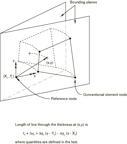
Let P 0 ( X 0 , Y 0 ) be a fixed point in one of the bounding planes, as shown in Figure 1. The length of the fiber between P 0 and its image in the other bounding plane is t 0 + Δ u z , where t 0 is the length of this fiber in the initial configuration and Δ u z is the change in length of this fiber. Δ u z is the value of degree of freedom 3 at the reference node of the element.
Figure 1. Generalized plane strain element.
The reference node should be the same for all elements in any given connected region so that the bounding planes are the same for that region. Different regions may have different reference nodes. Since the bounding planes are rigid, the length of a fiber at any other point ( x , y ) in the element is
t = t 0 + Δ u z + Δ ϕ x ( y - Y 0 ) - Δ ϕ y ( x - X 0 ) , Δ ϕ x = ( Δ ϕ x ) | 0 + ( Δ ϕ x ) 1 , Δ ϕ y = ( Δ ϕ y ) | 0 + ( Δ ϕ y ) 1 ,where ( Δ ϕ i ) | 0 ; i = x , y , are the initial values of Δ ϕ i , specified by the user; and ( Δ ϕ i ) | 1 are the degrees of freedom 4 and 5 at the reference node of the element.
The thickness direction logarithmic strain is
ε z z = ln ( t t 0 ) .The first variation of thickness direction strain is, therefore,
δ ε z z = δ t t , δ t = - Δ ϕ y δ x + Δ ϕ x δ y - x δ Δ ϕ y + y δ Δ ϕ x + δ Δ u z ;and the second variation is
d δ ε z z = d δ t t - δ t d t t 2 ,d δ t = - δ x d Δ ϕ y + δ y d Δ ϕ x - d x δ Δ ϕ y + d y δ Δ ϕ x .